Rebuilding my thesis workflow with Cursor

Galaxies are systems of components

The Milky Way is a disk galaxy. Most of its visible stars lie in a flattened, rotating stellar disk that also contains gas and dust. The central few kiloparsecs contain a denser, more nearly spheroidal bulge. Both components are embedded in a much larger dark matter halo, which extends well beyond the visible edge of the galaxy and contributes substantially to the gravitational field.

These components are useful idealizations rather than rigid pieces. The disk is not a smooth, featureless sheet. It develops spiral structure, in which stars and gas collect into rotating patterns, and it may form a bar, an elongated concentration of stars that crosses the center of the galaxy. Bars and spiral arms redistribute angular momentum and can alter the density and velocity structure of the disk. The bulge and dark halo respond to the same gravitational field, so the evolution of one component cannot generally be separated from the others.

Much of galactic dynamics is therefore a problem of controlled model construction. We specify a disk, bulge, and halo; assign each component a population of orbits; and ask how the combined system evolves. If the initial model is not close to equilibrium, the galaxy will rearrange itself, occasionally violently. Bars, spiral structure, or waves that form because the disk was initialized incorrectly are not evidence about galactic dynamics. They are evidence that the initial conditions were poor.

GalactICS was developed to address this problem. It constructs self-consistent disk-bulge-halo models by tying the density of each component to a distribution function in the combined gravitational potential. The full problem is axisymmetric and involves several families of orbits. For this first reconstruction I begin with the simplest nontrivial component: a spherical, isotropic dark matter halo with an NFW density profile. The geometry is simple enough that every stage of the calculation can be inspected, while the numerical questions are the same ones that reappear in more complicated galaxy models.

From an equilibrium model to an N-body experiment

An N-body simulation does not normally represent every star or dark matter particle individually. A simulation particle is a Monte Carlo sample from an underlying distribution in phase space. It carries mass and occupies a point in six-dimensional position-velocity space. The initial-condition code determines which points should be sampled. The N-body code then advances those samples under their mutual gravity.

The distinction between these two stages is important. GalactICS builds the equilibrium model. It solves for the gravitational potential and samples positions and velocities from the assumed distribution functions. It does not evolve the galaxy. The evolution is handled here by a separate package developed for this post, ntropy, which computes self-gravity, integrates the particle trajectories, and measures whether the sampled system remains close to the intended equilibrium.

The spherical halo is a useful test because failure is easy to recognize. The sampled density should reproduce the target NFW profile. The velocity distribution should agree with the isotropic distribution function. The enclosed mass should generate the expected circular-speed curve. After several billion years of self-gravitating evolution, the halo should still resemble the object that was sampled at the beginning.

Equilibrium is a phase-space statement

The central object in collisionless stellar dynamics is the distribution function,

It gives the mass density in phase space. In the collisionless limit, stars and dark matter particles move through the smooth gravitational field without undergoing frequent two-body encounters. The distribution function then obeys the collisionless Boltzmann equation,

The ordinary density is obtained by integrating over velocity, and the density generates the gravitational potential through Poisson’s equation:

The distribution function determines the density, the density determines the potential, and the potential determines the orbits on which the distribution function must remain steady. This is why matching a density profile is not sufficient. Two particle systems can have the same density at one instant and evolve very differently if their velocities sample different orbit populations.

How GalactICS represents the components

For an axisymmetric stellar disk, GalactICS uses an approximate three-integral distribution function. It is written schematically as

where E is the orbital energy, Lz is the angular momentum about the symmetry axis, and Ez describes the vertical motion. The dependence on Lz associates a star with a guiding-center radius. The radial and vertical energies describe oscillations about the corresponding circular orbit. GalactICS tabulates the orbital frequencies and iteratively corrects the distribution function so that its velocity integral recovers the target disk density.

The halo considered here is simpler. It is spherical, so its smooth density depends only on radius, and isotropic, so the velocity distribution has no preferred direction. Under these assumptions the distribution function depends only on the relative binding energy,

The reduction from f(E,Lz,Ez) to f(E) removes the complications associated with disk geometry while retaining the central equilibrium problem. It is therefore the natural place to test the rewritten potential solver, distribution-function calculation, particle sampler, force code, and time integrator.

The NFW halo and Eddington inversion

The target halo follows a truncated Navarro-Frenk-White profile. Before the outer taper is applied, the density has the form

The profile has a central cusp and approaches an r^-3 decline at large radius. Its total mass diverges logarithmically if it is extended to infinity, so a finite model requires a controlled truncation. The truncation defines a bound system with finite mass and avoids placing a sharp numerical edge at the outer boundary.

A density law specifies where the mass is, but not the velocities required to support it. For a spherical isotropic system, Eddington inversion recovers the distribution function from the density expressed as a function of the relative potential:

The density is an integral projection of the distribution function over velocity. Eddington’s formula reverses that projection. GalactICS tabulates f(E), draws radii from the target mass profile, and samples velocities that are consistent with the local potential and escape speed. The result should be a Monte Carlo realization of an equilibrium orbit population rather than a density profile with velocities attached afterward.

Sampling and validating the halo

The calculation proceeds in four stages. First, the model parameters and numerical grid are specified. Second, the Python dbh backend solves Poisson’s equation and constructs the energy tables required for the halo distribution function. Third, an OpenMP sampler draws the particle positions and velocities. Finally, ntropy loads those particles and performs the force and stability tests.

The initial diagnostics use 10,000 particles. This is still small by the standards of galaxy simulation, but it is large enough to resolve the radial structure and expose the scaling of the force algorithms while leaving an exact pairwise calculation within reach.

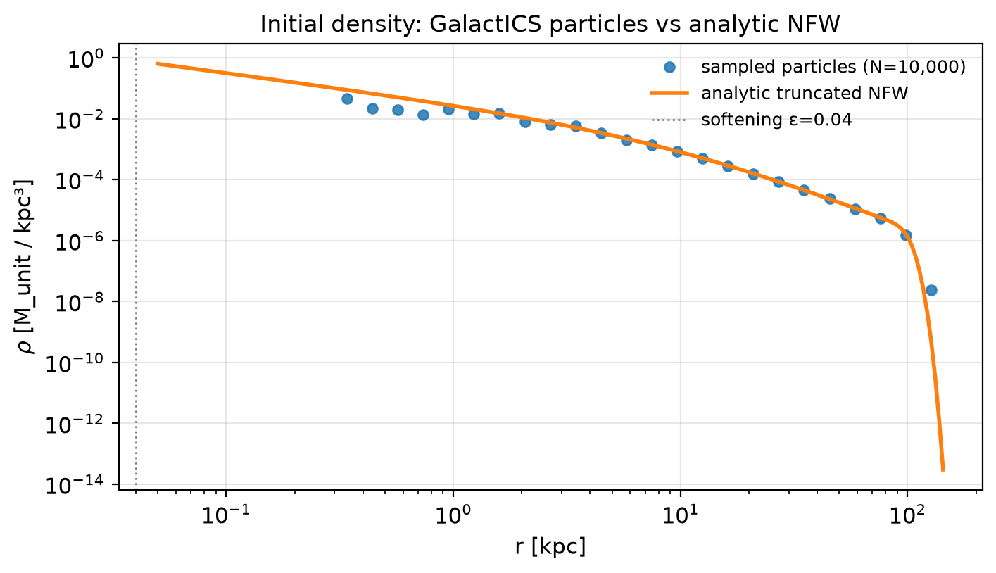
Figure 1 shows that the sampled density follows the target profile over the resolved radial range. The innermost bins are sensitive to finite sampling and force softening, while the outer bins contain fewer particles and therefore show more scatter. The important result is that there is no broad systematic offset between the particle realization and the analytic model. The potential solve, energy table, units, and radial sampler are mutually consistent.

The density test does not by itself establish equilibrium. Figure 2 tests the velocity sampling. The binding-energy distribution follows the range populated by the tabulated distribution function, while the radial velocity dispersion changes smoothly with radius. In particular, the outer halo is dynamically colder than the inner halo, as expected for a finite bound system. These diagnostics would expose a sampler that reproduced the density but assigned velocities from an unrelated prescription.

Figure 3 compares cumulative quantities. In a spherical system the circular speed is related to the enclosed mass by v_c^2=GM(<r)/r. This is the speed of a hypothetical circular orbit in the spherically averaged potential; it is not the mean tangential speed of the sampled halo particles. An isotropic halo is not made of circular orbits. It has no preferred velocity direction and is supported by a mixture of radial, tangential, and eccentric trajectories, with equal velocity dispersions in the three directions. The modest deviations between the sampled and analytic circular-speed curves are therefore not evidence of anisotropy or disequilibrium. They follow from finite-particle noise in the enclosed mass, radial binning, and the relatively small number of particles at the innermost and outermost radii. What matters is that the particle curve follows the analytic shape without a coherent offset. Together, the two panels show that the sampled realization generates the intended radial gravitational field.

The N-body problem

Once the initial conditions have been sampled, GalactICS has completed its part of the calculation. The N-body code must repeatedly compute the gravitational acceleration, advance the phase-space coordinates, and decide when the force field must be updated. The dominant numerical choices are the force approximation and the time integrator.

With Plummer softening, the direct acceleration on particle i is

Direct summation is useful as a reference because it introduces no far-field approximation. Its cost is proportional to N^2. Doubling the particle number produces roughly four times as many pair interactions, which makes the method unsuitable for the repeated force evaluations required by a large simulation.

Barnes-Hut gravity

The Barnes-Hut algorithm replaces the distant particle distribution with a hierarchy of approximate sources. The simulation volume is enclosed by a root node and recursively divided into octants. Each occupied node stores its total mass, center of mass, and spatial extent. During a force calculation, a distant node can be treated as a single monopole; a nearby node is opened and its children are examined.

The opening angle theta controls this decision. Smaller values open more nodes and approach the direct calculation. Larger values accept coarser approximations and reduce the cost of the tree walk. The appropriate value must be measured for the particle distribution and force accuracy required by the experiment.

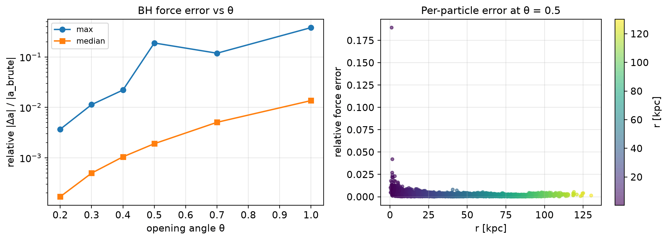
Figure 4 shows the expected accuracy-speed tradeoff. The force errors increase as theta is relaxed because larger tree nodes are accepted as monopoles. The distribution of errors is also more informative than a single mean value: most particles can have small errors while a small number of particles near awkward node boundaries have much larger errors. The notebook therefore reports several error statistics and uses direct summation as the calibration standard.

A readable reference and a compiled backend

I first tried a Python Barnes-Hut implementation. It remains useful because the recursive tree construction and opening rule are easy to inspect, and it provides an independent reference for the optimized path. It is not fast enough for thousands of repeated force evaluations. Moving the same monopole tree construction and walk into a compiled C kernel produced an approximately two-order-of-magnitude speedup over the Python implementation in the notebook benchmarks. That is the difference between a force calculation that is useful for inspection and one that can serve as the inner loop of a multi-gigayear integration. The two implementations are still compared for numerical agreement, and the Python path is retained as an executable reference rather than discarded after optimization.

Figure 5 illustrates why asymptotic scaling is not the whole performance story. At small particle number, vectorized direct summation can compete with or beat a tree because tree construction and traversal have fixed overhead. As N increases, the quadratic direct calculation grows much more rapidly and the Barnes-Hut advantage becomes clear. The useful crossover is a measured property of the implementation and hardware, not a consequence of writing O(N log N) next to the algorithm.

Figure 6 separates the two costs hidden inside a Barnes-Hut force call. The build time is nearly independent of theta, since the same tree is constructed before the walk begins. The walk becomes cheaper as theta increases because fewer nodes are opened. The corresponding increase in force error makes clear that tree persistence and opening-angle selection are separate optimizations: one reduces how often the hierarchy is rebuilt, while the other changes how aggressively it is approximated.

Figure 7 puts the backend choices on a common scale. The Python tree is valuable for verification but is not competitive as the production force kernel. The compiled tree removes that language overhead, while direct summation remains the exact small-N reference. Keeping all three paths makes it possible to distinguish an algorithmic error from an optimization error.

Distributing the force calculation

The next problem is to distribute the particles across CPU cores and, eventually, across nodes. A random assignment would balance the number of targets, but each rank would own particles scattered throughout the halo. Its spatial bounding box would span most of the system, memory access would have poor locality, and a local-tree exchange would tend to import nearly the entire remote particle set.

The code instead assigns each particle a Morton, or Z-order, key. The position is quantized on a three-dimensional grid and the bits of the x, y, and z coordinates are interleaved to form a single integer. Sorting by this key traces an approximate space-filling curve through the volume. Morton ordering is simpler than the Peano-Hilbert curve used by GADGET-2, but it serves the same purpose: nearby regions of space tend to remain nearby in the sorted array.

Figure 8 shows how a multidimensional position is converted into a sortable one-dimensional key. The curve occasionally jumps between regions, so locality is not exact. Nevertheless, particles that share the leading bits of their coordinates occupy the same large spatial cells and appear in contiguous sections of the ordering. This is sufficient to build compact domains with a simple sort.

Figure 9 applies the ordering to the halo rather than to an ideal grid. Consecutive stretches of the curve pass through coherent regions of the particle distribution. A contiguous split of the sorted array therefore gives each MPI rank a spatially concentrated set of target particles, in contrast to a random split in which every rank samples the full halo.

Figure 10 shows the resulting domains in projection. They are not simple rectangular boxes, since the Z-order curve can enter and leave a projected region, but they remain substantially more coherent than a random assignment. The domains give each rank a compact target set and provide the geometry needed to decide which remote tree nodes must be imported.

In the local-tree path, each rank builds a tree over its own particles and exchanges a Local Essential Tree with its peers. Distant remote structure can be represented by monopoles, while nearby structure is opened to leaves. A centrally concentrated halo is a difficult case because projected domain boxes overlap near the center. If the exchange degenerates and imports nearly every remote leaf, the code falls back to a replicated full-tree walk rather than duplicating near-direct work on every rank.

Figure 11 shows that the scaling is not monotonic. Additional MPI ranks reduce the number of targets handled by each process, but they also increase communication and may duplicate tree work. OpenMP threads share memory within a rank and avoid some of this communication, although thread scaling eventually saturates. The best configuration is therefore a measured balance between ranks and threads. The plot is a property of this machine, particle count, and implementation, not a universal prescription.

Time integration and the structure of the equations

The force calculation gives the instantaneous acceleration. The integrator determines how those accelerations are accumulated over billions of years. A collisionless N-body system is Hamiltonian. Its exact evolution preserves the symplectic geometry of phase space and, for an isolated system with a time-independent Hamiltonian, conserves total energy.

A symplectic integrator preserves that geometric structure, but it does not conserve the original Hamiltonian exactly. At fixed timestep, it can usually be interpreted as following the exact solution of a nearby Hamiltonian. Its energy error is therefore often bounded and oscillatory rather than steadily secular. “Symplectic” does not mean “zero energy drift.” A timestep that is too large can still produce a large bounded error, while changing or tiered timesteps, an approximate Barnes-Hut force, changes in the tree topology, and floating-point accumulation can all introduce a measurable secular component.

Euler and Leapfrog 1

The explicit Euler method advances positions and velocities using derivatives evaluated at the beginning of the step:

Euler is first-order accurate and requires one force evaluation. It is not symplectic. The position and velocity updates are both based on the old state, so the map systematically distorts the Hamiltonian flow.

The first-order leapfrog option in ntropy is symplectic Euler, implemented as a kick followed by a drift:

Leapfrog 1 has the same formal order and force-evaluation count as Euler. The only visible change is that the drift uses the updated velocity. That ordering makes the map symplectic. It can still show a substantial energy offset or an asymmetric oscillation at finite timestep, but it generally avoids the systematic phase-space contraction or expansion produced by explicit Euler.

RK2 and Leapfrog 2

The explicit midpoint Runge-Kutta method first estimates the state halfway through the interval:

and then uses the midpoint derivative for the full update:

RK2 is second-order accurate and uses two force evaluations in this implementation. It is a good general-purpose integrator, but it is not symplectic.

The second-order leapfrog method uses the velocity-Verlet, or kick-drift-kick, sequence:

RK2 and Leapfrog 2 have the same formal order and the same force-evaluation count. The important distinction is geometric. Leapfrog 2 is symplectic and time-reversible at fixed timestep for the separable gravitational Hamiltonian; explicit midpoint RK2 is neither. Leapfrog therefore tends to keep the long-term energy error within a bounded envelope, whereas RK2 can accumulate a secular bias even when its short-time trajectory error is comparable.

Figure 12 should be read as two like-for-like comparisons. Euler and Leapfrog 1 are both first-order methods with one force evaluation per step; the symplectic ordering substantially improves the long-term behavior, although Leapfrog 1 still exhibits finite-timestep energy error. RK2 and Leapfrog 2 are both second-order methods with two force evaluations; Leapfrog 2 keeps the error more tightly bounded, while RK2 develops a clearer secular component. The symplectic curves are not perfectly flat. Their residual drift reflects the finite step, approximate tree force, numerical roundoff, and the fact that practical tiered stepping is not an exactly fixed-step symplectic map.

Individual and tiered timesteps

A single global timestep is inefficient for a halo. Particles near the center experience larger accelerations and shorter orbital times than particles in the outskirts. A timestep small enough for the center forces slowly evolving outer particles to receive unnecessary force updates. A timestep chosen for the outskirts under-resolves the center.

The tiered integrator estimates an ideal timestep for each particle using the GADGET-style criterion

where epsilon is the particle softening length, |a| is the acceleration magnitude, and eta controls the accuracy. The ideal values are quantized into power-of-two bins,

Particles in bin zero are active on every fine substep. Particles in bin one are active on every second substep, particles in bin two on every fourth substep, and so on. The hierarchy preserves regular synchronization points for MPI communication. The code also limits a particle to a one-bin change at each update so that the timestep does not oscillate abruptly between very fine and very coarse values.

The force code must support active target subsets for this scheme to save work. Accelerations are recomputed for active particles and cached for inactive particles. Without that connection between the integrator and the force backend, individual timestep metadata would add complexity without reducing the dominant force cost.

Figure 13 shows the expected tradeoff. Smaller base timesteps and more restrictive values of eta place more particles in fine bins and reduce the integration error, but increase the number of active-particle force evaluations. The useful operating point depends on the observable and the duration of the simulation. A short equilibrium screen does not require the same tolerance as a ten-billion-year measurement of bar pattern speed.

The five-billion-year test

The long integration uses a mass-preserving subset of 4,096 particles so that the optimized implementation can be compared directly with the inspectable Python Barnes-Hut reference over a complete multi-gigayear evolution. The Python implementation becomes prohibitively slow as the particle count grows, so the reduced-N experiment is a validation choice rather than a statement about the practical scale of isolated-galaxy simulations.

Production isolated-galaxy simulations routinely contain millions to hundreds of millions of particles. The GPU force and integration paths developed alongside this work are intended for that regime and scale to those particle counts on scientifically useful timescales on the tested hardware. I will present those optimizations and large-N benchmarks in a separate post. Here, the smaller realization keeps the end-to-end physics, force, and integrator comparisons anchored to a transparent Python baseline.

The main test has two principal diagnostics. The density profile should remain close to its initial form, apart from finite-particle noise and the small relaxation expected from softening and force approximation. The total energy error should remain controlled. A broad contraction or expansion would indicate a problem with the sampled distribution function, the force calculation, the timestep, or some combination of the three.

Figure 14 is the end-to-end result. The final density remains close to the initial NFW realization over most of the resolved halo, and the energy error remains bounded at a level consistent with the chosen force and timestep settings. The deviations in the least populated radial bins are not unexpected for a 4,096-particle realization. More importantly, the halo does not undergo a coherent numerical collapse or expansion. The distribution-function sampler and N-body solver describe approximately the same equilibrium system.

The relationship to GADGET-2

ntropy is not a production cosmological code, and the comparison with GADGET-2 is architectural rather than competitive. GADGET-2 is useful here because it shows how the same numerical problems are organized in a mature, massively parallel particle code: hierarchical gravity, a space-filling-curve domain decomposition, hybrid parallelism, symplectic integration, and adaptive individual timesteps.

The present implementation uses a monopole Barnes-Hut tree rather than TreePM, Morton ordering rather than a Peano-Hilbert curve, and a simplified Local Essential Tree exchange. It uses MPI across processes and OpenMP within a node. Its leapfrog and power-of-two timestep hierarchy follow the same broad numerical logic. The purpose of these additions is not to reproduce every feature of GADGET-2, but to bring a small validation code under the same disciplines of force calibration, locality-aware decomposition, conservation testing, and measured scaling.

Reconstructing GalactICS

GalactICS is also a useful example of scientific software archaeology. The original implementation combines Fortran common blocks, C samplers, interactive executables, positional input files, and makefiles that encode the scientific workflow. The numerical ideas are sophisticated, but the interfaces assume that the user already understands which files must exist and in which order they must be generated.

The old Milky Way makefile contains a concise final construction step:

galaxy: disk bulge halo
	cat disk bulge halo > galaxy

By the time this command is reached, the potential has been solved, the distribution functions have been tabulated and corrected, and the individual components have been sampled. The final act of galaxy construction is simply to concatenate the particle files.

The rewrite began as a typed Python interface around this workflow. It now includes a native Python physics backend, OpenMP particle sampling, compiled and GPU force experiments, campaign tools, diagnostics, and a substantially larger test suite. The original Fortran and C sources remain in the repository as a reference implementation.

What Cursor changed

Cursor made the mechanical reconstruction much faster. It helped separate the modern packages from the legacy source, port numerical routines, propagate interface changes, write C-extension wrappers, create benchmark workers, and expand the tests. Once the numerical architecture was specified, it could implement several variants of a method and connect them to the same diagnostics in a short period of time.

The important omissions were scientific rather than syntactic. Early versions did not recover all of the halo-first and disk-distribution workflows used in my thesis. The first N-body implementation used poor integration defaults. Parallel paths sometimes duplicated work, and a tree method could appear more sophisticated while running more slowly than a direct calculation at the particle counts being tested. None of these problems was obvious from the fact that the code executed successfully.

The useful role of expertise was to specify the invariants and comparisons: the sampled density and distribution function, the direct force reference, agreement between Python and compiled kernels, bounded long-term energy error, spatially coherent MPI domains, and stability over several billion years. Cursor accelerated the implementation of those tests. It did not decide which tests made the calculation scientifically meaningful.

Where this goes next

At the beginning of this post, I framed the project as an attempt to apply recent advances in AI to the foundations of galactic dynamics. Cursor was useful in the first sense: it accelerated the reconstruction, testing, and optimization of the classical simulation pipeline. The more interesting next step is to apply modern machine-learning methods to the scientific problem itself.

The NFW halo is the baseline rather than the final model. The larger objective is to return to live disk-bulge-halo galaxies and study the much richer six-dimensional phase-space structure that develops as they evolve. Bars, spiral structure, bending waves, resonances, and disequilibrium are not described completely by a density image or a small collection of summary statistics. They appear as structured populations of orbits whose relationships change over time.

Recent advances in representation learning, generative modeling, and sequence architectures create new ways to ask whether those structures can be learned directly from particle data. A model might identify departures from equilibrium, organize simulations by their orbital structure, connect initial conditions to later morphology, or discover latent coordinates associated with the growth of bars and spiral patterns. Those experiments will be the subject of later entries in this series.

They require a trustworthy classical pipeline first. A representation model trained on unstable initial conditions may learn the artifacts of a poor distribution function, force approximation, or timestep. Before asking AI to reveal new structure in an evolving galaxy, the underlying simulation must have errors that are already understood.

Code and notebook

The current implementation is available on the main branch of PyGalactICS. The end-to-end calculation and the figures in this post are generated by notebooks/nfw_halo_walkthrough.ipynb. The corresponding algorithm notes are collected in the GalactICS pipeline documentation.

References

1. Bauer, J. S., Widrow, L. M., & Erkal, D. (2018). Disc-Halo Interactions in ΛCDM.
2. Bauer, J. S., & Widrow, L. M. (2018). Can Stellar Discs in a Cosmological Setting Avoid Forming Strong Bars?
3. Kuijken, K., & Dubinski, J. (1995). Nearly Self-Consistent Disk-Bulge-Halo Models for Galaxies.
4. Widrow, L. M., Pym, B., & Dubinski, J. (2008). Dynamical Blueprints for Galaxies.
5. Navarro, J. F., Frenk, C. S., & White, S. D. M. (1996). The Structure of Cold Dark Matter Halos.
6. Barnes, J., & Hut, P. (1986). A hierarchical O(N log N) force-calculation algorithm.
7. Springel, V. (2005). The cosmological simulation code GADGET-2.
8. Binney, J., & Tremaine, S. (2008). Galactic Dynamics, 2nd ed.