Vision Transformers Down Memory Lane (Part 1)

Image: Osaka Castle seen through some fall foliage in November, 2023.

An Amateur Photographer’s Problem

In 2022, I picked up photography as a hobby. I was traveling a lot for work, and wanted a way to remember the places I went. Looking at my own photography takes me back to the moment I captured the picture, and is fun to do over a beer. However, as any amateur photographer will attest, the vast majority of pictures you take don’t turn out quite like you envisioned (or maybe I’m just really bad). As a result, the photographer has to sift through large amounts of imagery to find a good set of pictures to edit and share.

In this blog post, I wanted to do some initial exploration on whether I could use recent advances in image representations to create random samples of images that represent a diverse body of photography. Low-dimensional representations, commonly called embeddings, make unstructured data queryable. LLM Retrieval Augmented Generation workflows, for example, use learned embeddings of source text and queries to identify relevant documents.

I will explore with the reader a class of models called vision transformers. Using these models, I will create different representations for a sample of my photography, cluster the representations, and pull out a core set of images. In a future blog post, I will turn this into an application to explore the photo space a bit more, but for now, we turn our attention to the stated problem. After a brief overview of vision transformers, I will discuss the data, the types of embeddings considered, and present the results of my clustering analysis. All of the code for this project can be found at: https://github.com/bauerj4/photography-analysis. I have licensed it as Apache 2.0, so please re-use in whatever way you wish.

What Are Vision Transformers?

Image processing since the early 2010s has largely been the domain of Convolutional Neural Networks (CNNs). Advances in hardware, notably the advent of GPU computing, alongside these algorithmic advancements were responsible for a boom in performance on visual tasks. While CNNs saw some application in natural language processing, contemporary deep learning approaches for text frequently relied on recurrent approaches like LSTMs. In 2017, with the publication of Attention is All You Need by Vaswani and colleagues, NLP literature exploded with approaches using the new transformer architecture. The BERT architecture (Devlin et al. 2019) is an early example of how transformers could be used as encoders to create deeply contextual representations of unstructured data. I think it is fair to say that transformer architectures dominate in text understanding today. Being brief, some of the main reasons for the rapid adoption of transformers include:

Parallelization: In encoder / decoder setups, the encoder is not recurrent. With some clever masking techniques and teacher forcing, attentions can be computed in parallel in the decoder during training.
Long-Range Dependencies: Capturing information from distant parts of the input sequence is done explicitly in the attention mechanism.
Simplicity: The actual attention mechanism itself is a relatively straightforward sequence of matrix multiplications. In my opinion, this is much simpler than the state management systems employed by LSTMs.

Owing to these clear benefits, various authors attempted to employ a similar approach on images with initially limited success (Dosovitskiy et al. 2021). In 2021, a model introduced by Dosovitskiy and his coauthors at Google presents a viable competitor to CNN architectures, 4 years after Vaswani et al.’s contributions.

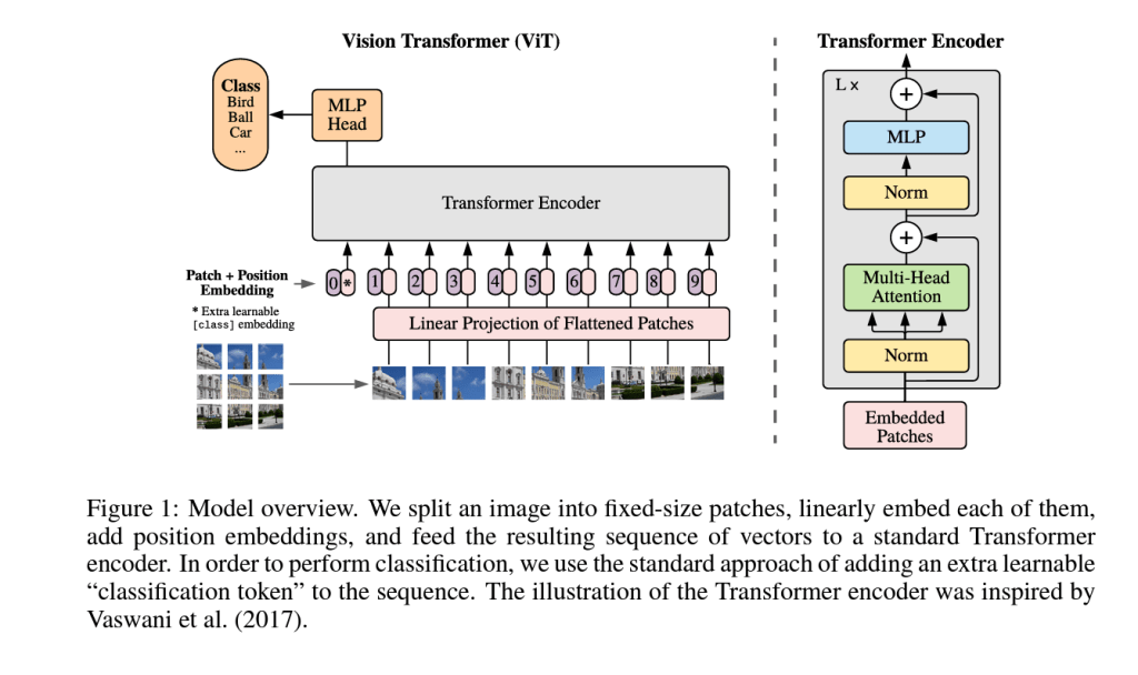
Figure 1: ViT architecture lifted from the 2021 paper by Dosovitskiy et al.

Figure 1 shows the ViT architecture with caption preserved. The key insight behind the design is the decomposition of the image into 16×16 “tokens” that are linearly projected into the model’s internal dimension. This is analogous to how the first step in many text approaches, the entire token vocabulary is projected down to the model dimension through a learned mapping. Said another way, every input token has a unique vector representation for the encoder. Another key feature of the design is the classification token prepended to the input sequence, which we will revisit later. The authors pre-train this model on classification tasks of increasing size in their paper (ImageNet (1.2 million images), ImageNet-21k (14 million images), and the in-house JFT-300M dataset (300 million images)) before fine-tuning it to achieve their final competitive results. Their paper also explores self-supervised pre-training by corrupting data at the patch level, but find that these results are not as performant as the supervised pre-training task. Although ViT refers to the architecture, the rest of this article will use ViT to mean a ViT model trained by Dosovitskiy et al. 2021’s approach.

Recently, the authors of DINO V2 (Oquab et al. 2024) have continued to expand on the self-supervised approach, although the core idea remains the same. The ingenuity of the DINO framework lies in a self-distillation approach where distorted input images are fed to student and teacher networks that share an architecture. By updating the teacher weights as an exponential moving average of the student’s learned weights, DINO has student learn the teacher’s outputs on a combination of patch and image level objectives. During this process, images are distorted like in Dosovitskiy et al. 2021 for the student network. There is an additional training objective to enforce the embeddings to be spread out within a batch. The paper is a really interesting read and I highly recommend it if you are interested in all of the complexities. In particular, I highly recommend looking at their ablation study.

For my purposes though, I am just interested in how the learned embeddings separate my photos. The authors of DINO V2 actually explore the classification capacity of this representation in their paper, and see some fairly impressive results by applying a k-Nearest Neighbors classifier. The fact that they are able to do this indicates that I should be able to separate my photos fairly well by using their embeddings. With this as motivation, I turn to my experiment.

Experiment Setup

In broad strokes, I break this section down into a discussion of the models I looked at, the data I used, the embeddings I extracted, and the clustering approach I built to create my sample of photos.

Models

Owing to their availability on Hugging Face, I chose to compare the vit-large-patch16-224-in21k and dinov2-large models. A few things to note about the models:

In both models, it is the last hidden state referred to in the model card that I use as the embedding.
Neither model is explicitly trained to have their hidden states to be directly comparable by the Euclidean distance.
The base model architecture for both ViT and DINO V2 have the same internal representation size of 1024, but the ViT model resizes images to a size of 224 vs 518 for DINO V2.
The patch size for DINO V2 is 14×14 vs 16×16 for the ViT model. In theory, this lets DINO V2 consider more local information.
The ViT model is pre-trained on a supervised task, so it is conceivable that I might get very different results than from using self-supervised embeddings. However, because of the differences in input and patch sizes, we won’t be able to unambiguously attribute performance differences to the training technique.

Data

I took approximately 700 6240 x 4160 pixel JPG files from one day of photography in Osaka, Japan. The images showcased are from me walking around the city that day, and represent diverse times, lighting, and subjects.

Embedding Approaches

For both ViT and DINO V2, I construct representations for my images using the following strategies:

Embedding Averaging: I take the arithmetic mean of all encoder outputs for each model. This includes an embedding for each patch and the classifier embedding resulting in a vector with the same dimension.
Embedding Concatenation: Even though positional encodings are included in DINO V2, sometimes concatenation is the best approach to avoid losing information. I look at clustering a single vector that concatenates the classifier embedding with all patch embeddings resulting in a… very large vector (approximately 200k-dimensional).
Classifier Embedding: Use as prescribed in the papers. I just use the first prepended classifier embedding to represent the entire image at the time of clustering.

Clustering Approach

To cluster the data, I use scikit-learn’s implementation of k-means. I choose this technique because the embeddings I explore are very high dimensional (~10³ for my smallest embeddings, and ~10⁵ for the largest), and things tend to be linearly separable in high dimensions. Since k-means enforces linear cluster boundaries, it can take advantage of this phenomenon. Furthermore, k-means will not be sensitive to photo density at specific places or settings. For each embedding approach, I look at a range of cluster counts and statistically evaluate cluster quality by looking at the Silhouette and Davies-Bouldin Indices. I choose one combination of embedding type and cluster count using the “Elbow Method” based on the sum of squared centroid distances. During the initial search, I set the n_init parameter, which re-runs the clustering a few times to achieve a better result, to 1 even though this is recommended to be higher in high dimensions. After the cluster quality search, when I create my image samples, I set it to 10.

Results

To describe my results, I first discuss the cluster quality analysis by embedding method, and then look at a few samples of the imagery from the clusters I create.

Cluster Analysis Metrics

Cluster quality can be measured by a variety of metrics. Choosing an appropriate number of clusters is as much of an art as a science, but I’ll guide myself this way. I consider:

Silhouette Score

The Silhouette Score is defined through a few simpler quantities. Define:

$a(i)={\frac{1}{|C_{I}|-1}}\sum_{j\in C_{I},i\neq j} d(i,j)$

where C is the cluster, i and j are indices of data in the cluster, and d is the (Euclidean) distance. This is the mean distance from i to all points in the same cluster. Also define:

$b(i)=\min _{J\neq I}{\frac {1}{|C_{J}|}}\sum _{j\in C_{J}}d(i,j)$

as the smallest mean distance to points in any cluster not containing i. From these, the SIlhouette Score can be defined as:

$s(i)={\frac {b(i)-a(i)}{\max\{a(i),b(i)\}}}$

You can intuitively think of this as expressing whether a point is closer to points in its own cluster or those of other clusters, and it ranges from [-1, 1] with 1 being a good clusterings. For more information, read the cited Wikipedia page. We use the scikit-learn implementation for the average Silhouette Score.

Davies-Bouldin Index

For the special case where we use the Euclidean distance, we can define:

$R_{x,y}=\frac{S_x + S_y}{M_{x,y}}$

where x and y are indices for clusters, S is average the Euclidean distance of points to the cluster centroid, and M is the distance between centroids for two clusters. Using this definition,

$D_x = \max_{x \neq y} R_{x,y}$

is the Davies-Bouldin Index for cluster x and the index we use is averaged over all clusters. Consequently, a low value is better because it means distances to the cluster centroids are small compared to inter-cluster distances. You can read more in the cited Wikpedia article.

Sum of Square Error

For every cluster, we also compute the sum of square distances to the centroid as its own metric. Commonly, this quantity is used to assist in picking the number of clusters through the “Elbow Method”.

Calculated Metrics

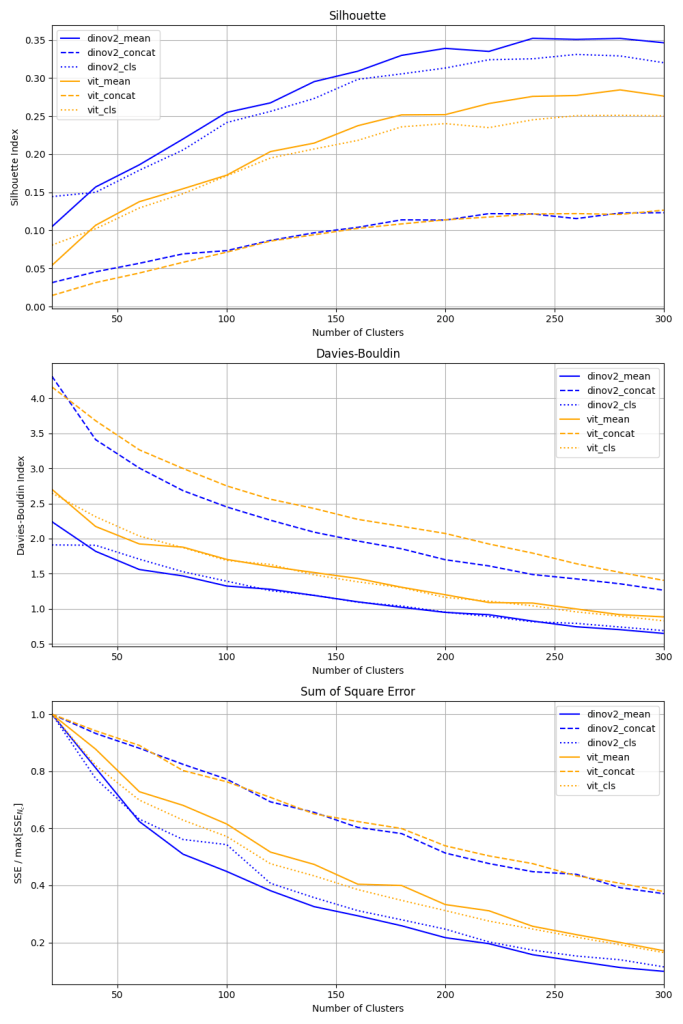
Figure 2: The metrics described above computed for each embedding type.

Figure 2 shows my analysis of varying the number of clusters and its effect on cluster quality metrics. Taking the Silhouette score for the various embedding approaches, it’s interesting to note that the concatenated methods do horrendously. DINO V2 seems to generate better clusters based on this index, and it does seem like averaging the patch-level embeddings provides benefit at higher numbers of clusters. Moving onto the Davies-Bouldin index, we see congruent results, although the benefit of averaging over patches is less pronounced with this metric. Turning to the sum of squares error (normalized by the max value), we see DINO V2 mean and classification embeddings capitalize more efficiently on the addition of additional clusters. The difference is large compared to the ViT model, which I was a little surprised by.

Applying the “Elbow Method” to this plot would suggest we pick our number of clusters somewhere around 120 for DINO V2. Furthermore, I use the Silhouette score to break the close tie between the classification and mean-aggregated vectors. One caveat to doing this is that these metrics rely on distances, and these vectors are not the result of an objective that explicitly encourages comparison by the Euclidean distance (except for the KoLeo loss mentioned in the DINO V2 paper). However, I choose to ignore this potential danger and proceed as described. Using the mean-aggregated embedding technique and 120 clusters, I re-run the clustering.

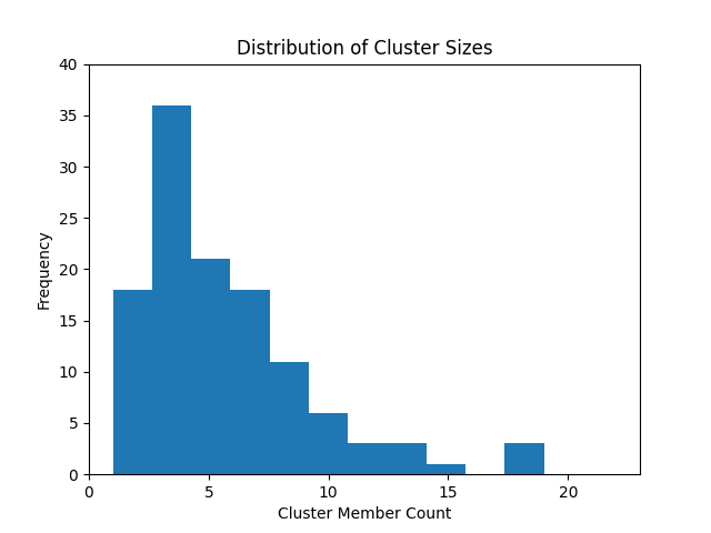
Figure 3: The distribution of the k-means cluster sizes for DINO V2 mean-aggregated vectors when the number of clusters is set to 120.

Figure 3 shows the distribution of cluster sizes for our preferred clustering method. The majority of clusters have fewer than 5 images, but there is definitely a right skew. However, this healthy mix of cluster sizes gives me confidence. With our candidate clustering and embeddings in hand, let’s look at some photography samples!

Generated Photo Samples

First, let’s have a look at a grid of 120 images.

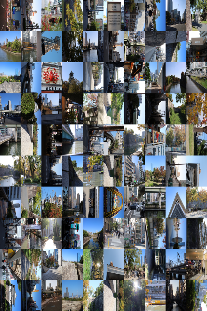
Figure 4: A sample of one picture from each of the 120 clusters of DINO V2 mean-aggregated embeddings.

Figure 4 shows a grid of single pictures taken from each of the clusters. Subjectively, this seems like a pretty uniform sample over the events of the day (I see you giant crab outside the かに道楽 (Kani Douraku)). While a lot of these wouldn’t necessarily be my favorite picture from each cluster, they are certainly relatively uniformly distributed in time and space. As a sanity check, let’s examine the contents of the largest cluster.

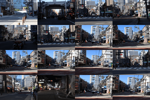
Figure 5: The largest cluster in the DINO V2 mean-aggregated clustering.

Figure 5 shows the content of (one of) the largest clusters containing 16 unique images. The vast majority of these were taken within minutes of each other. These are all street scenes with sidewalks and man-made objects in the foreground. Although the time of day is different for some of the pictures, the semantic content seems to be understood by DINO V2.

Just for completeness, I ran the clustering using the ViT mean-aggregated embeddings. While I wasn’t able to detect any subjective differences in quality at the 1 image per cluster level, my impression was different when I examined the largest clusters.

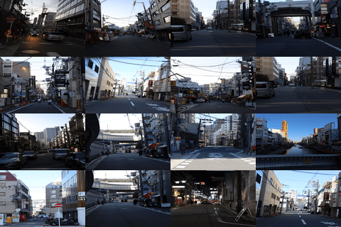
Figure 6: The largest cluster in the ViT mean-aggregated clustering.

Subjectively, Figure 6 shows me much more varied content than Figure 5. For example, the tight grouping of one particular alley shot in Figure 5 is not present in any of the top 10 largest clusters using ViT. Additionally, the cluster in Figure 6 shows a much broader range of lighting conditions. This may be captured in the higher sum of squares metric associated with this embedding technique. Finally, just for fun, I had a look at the largest clusters when I re-ran with the ViT concatenated embeddings.

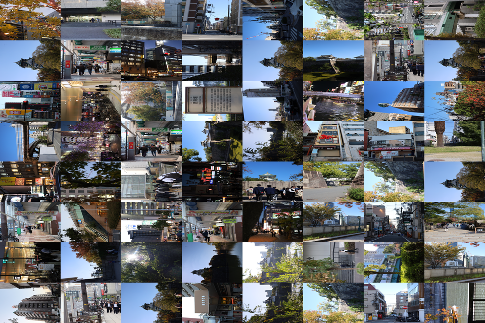
Figure 7: The largest cluster in the ViT concatenated-aggregated clustering.

This is almost comically bad. In addition to taking more than 15 minutes to cluster, the largest cluster for the concatenated approach has 79 members… (lol). If there’s a theme here, I can’t see it. I did try to cluster 201,728-dimensional vectors though, so this should be expected.

Thoughts and Conclusions

I think the key takeaway is that the vision transformer embeddings are very good at producing image separability based on semantic content. In particular, I was extremely impressed with the quality of the DINO V2 embeddings. While we can’t truly say this is an apples to apples comparison to a supervised ViT model due to the differences in input image size, the semantic understanding that is being extracted is truly impressive. The combination of input image sizes and training method clearly produce superior separability of the data based on various cluster metrics. I can also say that the cluster metrics do seem to generally correlate to subjective “quality” in the content of the clusters, making this a viable approach to explore further for productionalization. I am just amazed that I didn’t have to train a single model to achieve this quality.

As we look to the future where foundational models for imagery become more common, another key theme I will be paying attention to is how multimodal models develop from self-supervised methods. There is potential for true semantic understanding of how humans interact on the internet via social media if effective combination of language and visual understanding can be accomplished. In the meantime, I am very pleased with my experiment, and I think I have the beginnings of a solid photo shortlisting application. In my next post on this subject, I will build a web application around these models and a vector database, and show how I can deploy it using Docker. Thanks for reading, and I look forward to the discussion!

References

Vaswani, Ashish, Noam Shazeer, Niki Parmar, Jakob Uszkoreit, Llion Jones, Aidan N. Gomez, Lukasz Kaiser, and Illia Polosukhin. “Attention Is All You Need.” arXiv, August 1, 2023. https://doi.org/10.48550/arXiv.1706.03762.
Devlin, Jacob, Ming-Wei Chang, Kenton Lee, and Kristina Toutanova. “BERT: Pre-Training of Deep Bidirectional Transformers for Language Understanding.” arXiv, May 24, 2019. https://doi.org/10.48550/arXiv.1810.04805.
Dosovitskiy, Alexey, Lucas Beyer, Alexander Kolesnikov, Dirk Weissenborn, Xiaohua Zhai, Thomas Unterthiner, Mostafa Dehghani, et al. “An Image Is Worth 16×16 Words: Transformers for Image Recognition at Scale.” arXiv, June 3, 2021. https://doi.org/10.48550/arXiv.2010.11929.
“[1707.02968] Revisiting Unreasonable Effectiveness of Data in Deep Learning Era.” Accessed July 30, 2024. https://arxiv.org/abs/1707.02968.
“[2104.10972] ImageNet-21K Pretraining for the Masses.” Accessed July 30, 2024. https://arxiv.org/abs/2104.10972.
Oquab, Maxime, Timothée Darcet, Théo Moutakanni, Huy Vo, Marc Szafraniec, Vasil Khalidov, Pierre Fernandez, et al. “DINOv2: Learning Robust Visual Features without Supervision.” arXiv, February 2, 2024. https://doi.org/10.48550/arXiv.2304.07193.
Pedregosa, Fabian, Gaël Varoquaux, Alexandre Gramfort, Vincent Michel, Bertrand Thirion, Olivier Grisel, Mathieu Blondel, et al. “Scikit-Learn: Machine Learning in Python.” Journal of Machine Learning Research 12, no. 85 (2011): 2825–30.
“Silhouette (Clustering).” In Wikipedia, July 1, 2024. https://en.wikipedia.org/w/index.php?title=Silhouette_(clustering)&oldid=1231979269.
“Davies–Bouldin Index.” In Wikipedia, November 22, 2023. https://en.wikipedia.org/w/index.php?title=Davies%E2%80%93Bouldin_index&oldid=1186394772.

Jake's Blog